Payload Monte Carlo study
Continue the load-at-a-motor experiment: how much prescribed
payload weight can the fixed controller tolerate on the same waypoint mission?
Vary the payload mass used in F = m g, keeping its attachment at the
front-right motor, 77.8 mm forward and 77.8 mm right of the center, in the
motor plane. The QAV-R’s own mass, inertia,
geometry, motors, firmware, gains, and mission stay fixed.
The recorded batch contains 18 runs: nine completed missions (including the unloaded reference) and nine firmware crash disarms. The heaviest successful sample was 321.6 g; the lightest failed sample was 359.8 g. These are observations for this mission and controller, not an exact stability boundary. The plant models ground contact at landing points; motion after tipping is not a detailed airframe collision reconstruction.
Start with the recorded trajectories below. For a short hands-on check, run the zero-load reference in step 4. The complete batch is an optional longer experiment; you can replot its archived logs immediately using step 6.
1. Inspect the recorded flights
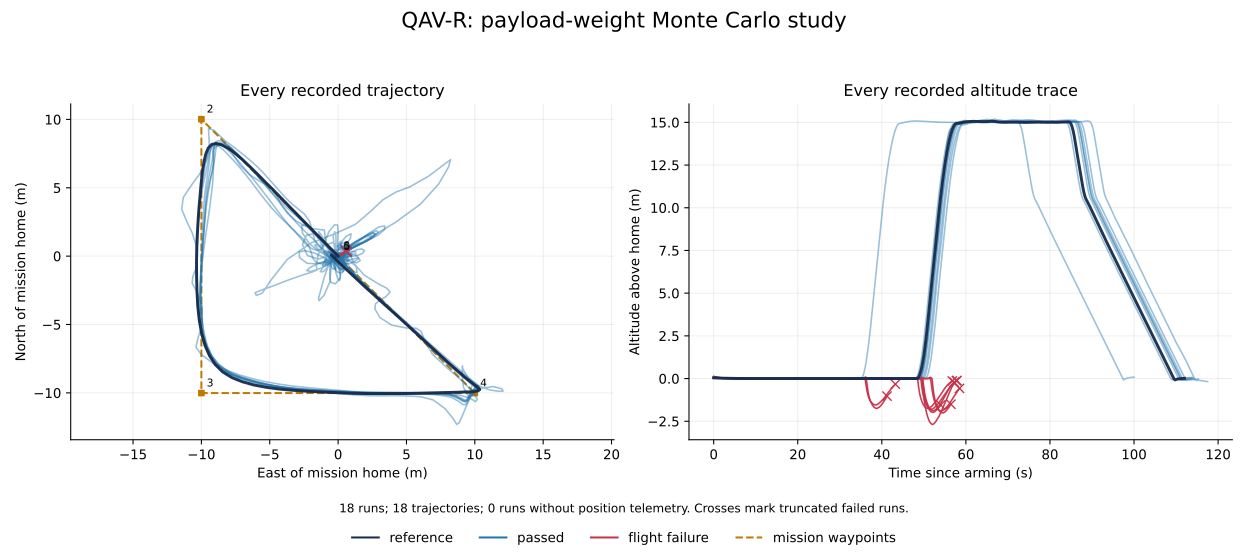
Every recorded trajectory is shown on common axes. The zero-load reference is dark, completed missions are blue, and flights stopped by a failure criterion are red. Select a mass to highlight that run; the other paths remain visible. Crosses mark the final sample of interrupted runs. Runs without position telemetry remain in the table.
Static plot of all trajectories and altitude traces
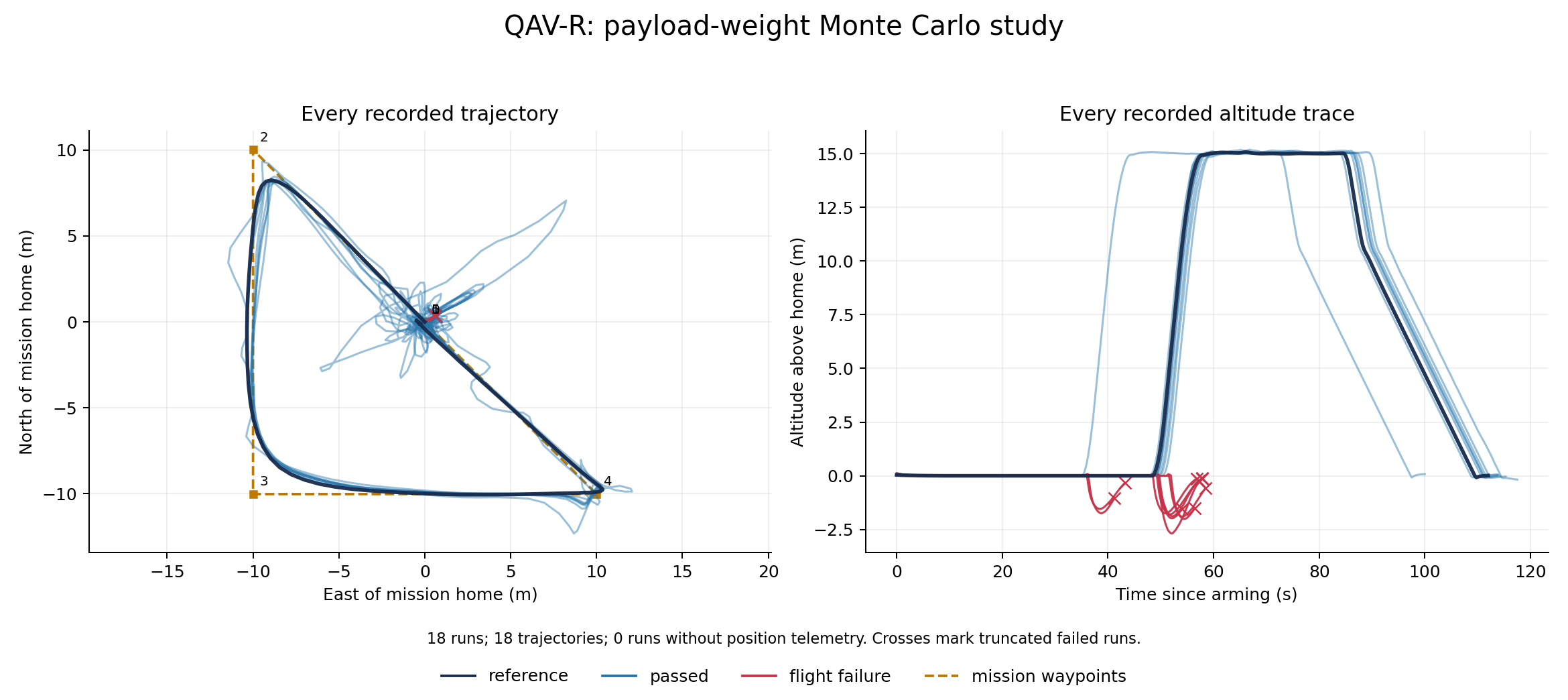
18 of 18 runs completed (including the nominal reference).
| Run | Payload mass (g) | Result | Peak armed tilt |
|---|---|---|---|
| reference | 0.0 | reference | 16.9° |
| payload-limit | 500.0 | flight failure | 179.2° |
| run-000 | 438.7 | flight failure | 179.0° |
| run-001 | 220.6 | passed | 27.5° |
| run-002 | 198.4 | passed | 23.4° |
| run-003 | 488.3 | flight failure | 178.8° |
| run-004 | 70.0 | passed | 15.3° |
| run-005 | 231.2 | passed | 28.9° |
| run-006 | 359.8 | flight failure | 179.5° |
| run-007 | 430.6 | flight failure | 179.2° |
| run-008 | 430.0 | flight failure | 178.6° |
| run-009 | 321.6 | passed | 40.9° |
| run-010 | 472.2 | flight failure | 179.1° |
| run-011 | 485.5 | flight failure | 178.9° |
| run-012 | 242.2 | passed | 28.8° |
| run-013 | 226.6 | passed | 28.6° |
| run-014 | 225.3 | passed | 27.3° |
| run-015 | 391.5 | flight failure | 179.0° |
Peak armed tilt includes takeoff and ground contact. The separate sustained-tilt stop criterion activates only after the vehicle has risen above 2 m. The firmware’s own crash check can disarm it before that height.
Download SVG · All trajectory data · Run manifest · Study settings and controller gains · Model library license
Which model produced these results?
Each trial extends the same FastDyn.QavrSidePayload model from the preceding
chapter and uses the environment’s pinned Rumoca compiler. The QAV-R geometry,
array-valued inertia, motor response, and selected controller gains stay fixed.
Only the prescribed payload mass changes. The run manifest records source and
compiler provenance alongside the measured results.
Generated zero-load QAV-R variant
within FastDyn;
model PayloadTrial
  import Vehicles;
  import Geodesy;
  import RigidBody;
  extends QavrSidePayload(
    bare_mass=0.5,
    payload_mass=0,
    attachment_b={0.07778174593052023, -0.07778174593052023, 0});
end PayloadTrial;
2. Understand the sampled quantity
The primary model exposes the scalar payload_mass in kilograms:
within FastDyn;

model QavrSidePayload "QAV-R with a downward load at its front-right motor"
  import Vehicles;
  import Geodesy;
  parameter Real payload_mass = 0.05
    "Payload mass used to prescribe its weight; payload inertia is omitted [kg]";
  // Independent coordinates stay writable as FMI parameters. These equal
  // {0.11 / sqrt(2), -0.11 / sqrt(2), 0} for the assumed QAV-R motor layout.
  parameter Real attachment_b[3] = {0.07778174593052023, -0.07778174593052023, 0}
    "Front-right motor (motor 1), from CG in body FLU [m]";

  extends Qavr(plant(external_force_b = force_b, external_moment_b = moment_b));

  Real force_world[3] "Prescribed payload weight in world NWU [N]";
  Real force_b[3] "Applied force expressed in body FLU [N]";
  Real moment_b[3] "Moment about vehicle CG in body FLU [N*m]";
equation
  // The load stays world-down when the aircraft tilts.
  force_world = {0, 0, -payload_mass * plant.gravity};
  force_b = transpose(plant.R) * force_world;
  moment_b = cross(attachment_b, force_b);
  // This is an external load, not an additional rigid body's inertial dynamics.
end QavrSidePayload;
At level attitude, a 50 g mass gives a downward force of 0.49 N and a positive body-FLU roll moment and pitch moment of approximately 0.0381 N m each. A 100 g mass doubles both. The force remains world-down as the aircraft tilts. Each trial compiles its own FMU so the load also reaches any derived expressions evaluated during compilation.
This study uses a zero-load reference, 16 uniformly sampled masses from
0 to 500 g, and an explicit 500 g upper-limit run. NumPy’s PCG64 generator
uses seed 462. The upper limit is 100% of the original 500 g vehicle
weight: payload_mass / vehicle_mass <= 1.0. At this endpoint the combined
static weight is equivalent to 1.0 kg under gravity. The uniform distribution
explores the selected range; it does not estimate how frequently real payload
masses occur.
This is the external-load approximation from the preceding chapter: changing
payload_mass changes the prescribed weight, not the vehicle’s inertial
mass. It does not simulate the payload’s swinging or acceleration-dependent
tension. Those require additional dynamics.
3. Predict the trend before running
More payload weight requires more total thrust and more unequal motor effort.
Let W = 0.50 * 9.8 be the original vehicle weight and P = payload_mass * 9.8
be the applied load. Balancing total thrust, roll, pitch, and yaw at level hover
for this square-X motor layout gives:
T1 (front-right, payload motor) = (W + 3 P) / 4
T2 (rear-left, opposite motor)  = (W - P) / 4
T3 (front-left) = T4 (rear-right) = (W + P) / 4
At 500 g of payload, the force is 4.90 N, with 0.381 N m of roll moment and the same pitch moment. The ideal allocation is 4.90 N, 0 N, 2.45 N, 2.45 N for motors 1–4. Motor 2 reaches zero thrust, leaving no room to reduce it further. This motivates testing the endpoint: transients and the fixed controller may lose control before or near that condition.
4. Run the experiment
Use your chosen environment:
fastdyn-config --base configs/copter462.toml \
  --overlay configs/models/qavr-side-payload.toml --output out/payload-base.toml
python utils/payload_study.py --config configs/monte-carlo/payload.toml \
  --run-config out/payload-base.toml --limit 1
The reference run should report:
[study] reference: payload 0.0 g
[study] reference: reference — Final mission item and landing confirmed
Remove --limit 1 to run the full batch. The runner resumes completed samples
in the same output directory and refuses to mix changed experiment inputs.
Choose a fresh output directory when changing the study or controller. Run one
batch at a time because the configured MAVLink ports are shared.
The runner snapshots the current model sources and generates each trial’s Modelica class. Edit the study TOML to change sweep settings; the runner replaces generated trial sources. Develop a different force law in a separately maintained model and validate it before automating its trials.
All persistent settings, including controller parameters, are in TOML:
# Payload range: 0 to 100% of the ORIGINAL vehicle mass (0 to 500 g).
# Attachment: motor 1, front-right, in body FLU.
# Same array-based model and selected gains as the load exercise.
[study]
title = "QAV-R: payload-weight Monte Carlo study"
seed = 462
samples = 16
distribution = "uniform"
attachment_b_m = [
    0.07778174593052023,
    -0.07778174593052023,
    0.0,
]
modelica_models_revision = "dfdb3294f61ab639a8a8be19611a1f69187a3ff7"
rumoca_revision = "21843c115cd4b4c7fa02011d18a6c1e501ebb387"
rumoca_version = "0.10.0"
mission = "virtuals/physics/flight_controllers/courbet/mavlink/copter_mission.waypoints"
vehicle_mass_kg = 0.5
max_payload_to_vehicle_mass_ratio = 1.0

[execution]
output = "out/payload-experiment"
# Optional: set to docs/book/assets/payload-study after reviewing a full batch.
publish = ""
wall_timeout_s = 150
monitor_port = 5565
max_tilt_deg = 60.0
tilt_duration_s = 1.0
max_altitude_m = 50.0

[parameters]
BRD_SAFETY_DEFLT = 0
FS_THR_ENABLE = 0
FS_GCS_ENABLE = 0
DISARM_DELAY = 0
EK3_SRC1_POSZ = 3
EK3_SRC2_POSZ = 3
EK3_SRC3_POSZ = 3
COMPASS_DEC = 0.0
COMPASS_AUTODEC = 0
ARMING_CHECK = 0
GUID_OPTIONS = 0
MOT_PWM_MIN = 1100
MOT_PWM_MAX = 1900
MOT_THST_EXPO = 0.5
MOT_THST_HOVER = 0.2
ATC_RAT_RLL_P = 0.04598495
ATC_RAT_RLL_I = 0.04598495
ATC_RAT_RLL_D = 0.00120043
ATC_RAT_PIT_P = 0.07421205
ATC_RAT_PIT_I = 0.07421205
ATC_RAT_PIT_D = 0.001949416
ATC_RAT_RLL_FLTT = 40.0
ATC_RAT_RLL_FLTD = 40.0
ATC_RAT_PIT_FLTT = 40.0
ATC_RAT_PIT_FLTD = 40.0
ATC_ANG_RLL_P = 4.5
ATC_ANG_PIT_P = 4.5
Expect a Modelica variant, compiled FMU, controller parameter file, run TOML,
console log, MAVLink log, and result.json for each trial. The publish
setting is optional and is empty by default, so your one-run check
does not replace the book’s archived results. Find the new figures under
out/payload-experiment/report/. To publish a reviewed full batch into this
book, set publish = "docs/book/assets/payload-study" before starting a fresh
output directory.
5. Interpret the outcomes
Every run starts fresh firmware and separate RAM files, then loads the same controller parameters. Completing the Copter mission requires the final item and landing confirmation. FastDyn and its separate helper processes are stopped before the next trial starts.
The experiment stops a flight if sampled tilt exceeds 60° across at least
1 s after becoming airborne, altitude exceeds 50 m, or the firmware
reports crash disarming. Tilt is acos(cos(roll) * cos(pitch)); this uses the
recorded MAVLink samples and does not certify behavior between samples.
A flight that arms but misses the completion deadline is mission incomplete. A compiler or startup failure is a run error. These labels distinguish an observed flight failure from an unavailable simulation; a timeout alone does not establish instability. Partial failed-run trajectories are retained.
A finite Monte Carlo sample can reveal failures at particular masses. It cannot prove an exact stability boundary or establish that every unsampled mass will work. To refine a transition, narrow the mass interval in TOML, use a new output directory, and repeat with the same controller.
6. Replot the archived logs
In your chosen environment, regenerate the plot from the book’s saved measurements:
python utils/monte_carlo_report.py \
  --config docs/book/assets/payload-study/runs.toml \
  --output out/payload-replot
The command reports the total number of runs, available trajectories, and runs without position telemetry. Both interactive and static figures include every available path, including interrupted flights.