Apply a load at the front-right motor

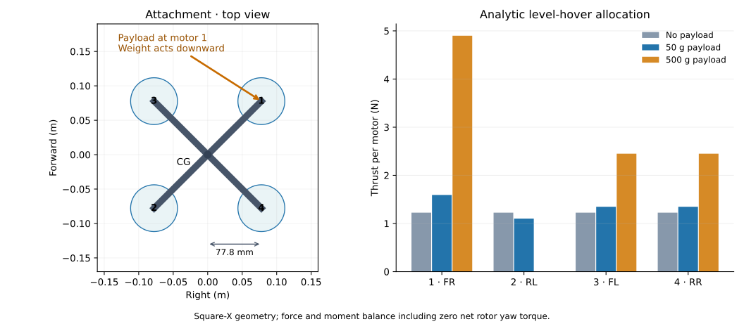
Use a 50 g payload mass to prescribe a 0.49 N downward force at the front-right motor (motor 1). In the assumed square-X layout, this is 77.8 mm forward and 77.8 mm right of the center, in the motor plane. The QAV-R’s mass and inertia stay at their original values. You will convert mass to weight, rotate the force into body coordinates, then compute its moment.

A downward load at motor 1 changes the hover thrust required from all four motors

1. Read the complete load model

within FastDyn;

model QavrSidePayload "QAV-R with a downward load at its front-right motor"
  import Vehicles;
  import Geodesy;
  parameter Real payload_mass = 0.05
    "Payload mass used to prescribe its weight; payload inertia is omitted [kg]";
  // Independent coordinates stay writable as FMI parameters. These equal
  // {0.11 / sqrt(2), -0.11 / sqrt(2), 0} for the assumed QAV-R motor layout.
  parameter Real attachment_b[3] = {0.07778174593052023, -0.07778174593052023, 0}
    "Front-right motor (motor 1), from CG in body FLU [m]";

  extends Qavr(plant(external_force_b = force_b, external_moment_b = moment_b));

  Real force_world[3] "Prescribed payload weight in world NWU [N]";
  Real force_b[3] "Applied force expressed in body FLU [N]";
  Real moment_b[3] "Moment about vehicle CG in body FLU [N*m]";
equation
  // The load stays world-down when the aircraft tilts.
  force_world = {0, 0, -payload_mass * plant.gravity};
  force_b = transpose(plant.R) * force_world;
  moment_b = cross(attachment_b, force_b);
  // This is an external load, not an additional rigid body's inertial dynamics.
end QavrSidePayload;

force_world is expressed in world north, west, up, so its negative Z component points down. attachment_b is expressed in body forward, left, up, so negative Y puts the attachment on the right. plant.R rotates body vectors to world coordinates; its transpose converts the world force into body axes. The force therefore stays world-down when the vehicle tilts.

The applied weight is payload_mass * plant.gravity. Its moment follows the familiar lever-arm relation:

[ M_b = r_b \times F_b. ]

With a level vehicle and the default 50 g payload mass:

force_b  = {0, 0, -0.49} N
moment_b = {0.038113, 0.038113, 0} N m

The moment is about the existing vehicle CG. Apply the force and moment once; there is no additional mass, CG shift, or inertia correction in this example.

2. See where the force enters the physics

The library template at the pinned revision sums its forces internally and does not yet expose external-load inputs. FastDyn keeps a local adaptation, modelica/FastDyn/QuadrotorWithExternalWrench.mo, of Vehicles.Templates.QuadrotorPlant. It adds two body-frame inputs and adds them to the force and moment sums before rigid-body integration:

  M_b = M_rotor + M_rate + M_ground_b + external_moment_b;
  F_b = F_ground_b + drag_b + {0, 0, T} + external_force_b;

The normal Copter and QAV-R models bind those inputs to zero. QavrSidePayload binds them to the force and moment computed above. Motor response, drag, ground contacts, and the rigid-body equations still come from the template design. This changes plant physics while preserving FastDyn’s PWM and sensor interface.

Complete quadrotor template with external-load inputs

within FastDyn;

// Adapted from Vehicles.Templates.QuadrotorPlant in modelica_models
// dfdb3294f61ab639a8a8be19611a1f69187a3ff7 (Apache-2.0).
// The only physics changes are two body-frame load inputs added to F_b/M_b.
// Keep this local adaptation until the upstream template exposes load inputs.
// Parameterized 6-DOF quadrotor plant model.
//
// Inputs:  4 motor angular velocities [rad/s]
// States:  rigid body pose/velocity plus motor speeds
//
// Internal frame uses local world Z Up and body axes Forward-Left-Up.
//
// Motor layout (ArduPilot Quad-X output order):
//   1: front-right  CCW   2: rear-left   CCW
//   3: front-left   CW    4: rear-right  CW

model QuadrotorWithExternalWrench
  parameter Real vehicle_mass = 2.0 "Total vehicle mass [kg]";
  parameter Real gravity = 9.80665 "Gravitational acceleration [m/s2]";
  parameter Real vehicle_ixx = 0.02166666666666667 "Body inertia xx [kg*m^2]";
  parameter Real vehicle_iyy = 0.02166666666666667 "Body inertia yy [kg*m^2]";
  parameter Real vehicle_izz = 0.04000000000000001 "Body inertia zz [kg*m^2]";

  extends RigidBody.RigidBody6DOF(
    mass = vehicle_mass,
    g = gravity,
    ixx = vehicle_ixx,
    iyy = vehicle_iyy,
    izz = vehicle_izz,
    p_start = {0, 0, ground_z - leg_z + initial_ground_clearance},
    qnorm_gain = 1.0
  );

  // Aerodynamic and actuator parameters
  parameter Real Ct = 8.54858e-6 "Thrust coefficient [N/(rad/s)^2]";
  parameter Real Cm = 0.016 "Rotor torque/thrust ratio [m]";
  parameter Real arm_length = 0.25 "Arm length [m]";
  parameter Real d = arm_length / sqrt(2.0) "Effective moment arm [m]";
  parameter Real Cl_p = -0.2 "Rolling moment coefficient per roll rate";
  parameter Real Cm_q = -0.2 "Pitching moment coefficient per pitch rate";
  parameter Real Cn_r = -0.1 "Yawing moment coefficient per yaw rate";
  parameter Real motor_thrust_scale[4] = {1, 1, 1, 1}
    "Per-motor thrust effectiveness multiplier for fault/robustness studies";
  parameter Real S = 0.1 "Reference area [m^2]";
  parameter Real CdA[3] = {0.06, 0.08, 0.12} "Body-axis drag area [m^2]";
  parameter Real linear_drag[3] = {0.12, 0.12, 0.18} "Low-speed body-axis drag [N/(m/s)]";
  parameter Real rho = 1.225 "Air density [kg/m^3]";
  parameter Real mag_world_enu[3] = {0.0, 0.21, -0.45}
    "Magnetic field in world ENU axes [Gauss]";

  // Ground contact (spring-damper)
  parameter Real ground_k = 3000 "Ground stiffness per contact point [N/m]";
  parameter Real ground_c = 150 "Ground normal damping per contact point [N*s/m]";
  parameter Real ground_tangent_c = 25 "Ground tangential damping per contact point [N*s/m]";
  parameter Real ground_z = 0.0 "World Z coordinate of the ground collision plane [m]";
  parameter Real initial_ground_clearance = 0.02 "Initial landing-leg clearance above the ground plane [m]";
  parameter Real leg_x = 0.17 "Landing contact X offset from CG [m]";
  parameter Real leg_y = 0.17 "Landing contact Y offset from CG [m]";
  parameter Real leg_z = -0.10 "Landing contact Z offset from CG [m]";

  // Motor first-order response
  parameter Real tau_up = 0.0125 "Motor spin-up time constant [s]";
  parameter Real tau_down = 0.025 "Motor spin-down time constant [s]";
  parameter Real motor_tau_eps = 1.0 "Smooth transition width for asymmetric motor lag [rad/s]";
  parameter Real motor_moment_map[3, 4] = [
    -d,   d,   d,  -d;
    -d,   d,  -d,   d;
   -Cm, -Cm,  Cm,  Cm
  ] "Motor thrust to body moment map";
  parameter Real rate_damping[3] = {
    4 * S * arm_length * Cl_p,
    4 * S * arm_length * Cm_q,
    4 * S * arm_length * Cn_r
  } "Body rate damping coefficients";

  model Motor
    parameter Real Ct = 8.54858e-6 "Thrust coefficient [N/(rad/s)^2]";
    parameter Real tau_up = 0.0125 "Motor spin-up time constant [s]";
    parameter Real tau_down = 0.025 "Motor spin-down time constant [s]";
    parameter Real tau_inv_mid = 0.5 * (1.0 / tau_up + 1.0 / tau_down) "Mean inverse motor lag [1/s]";
    parameter Real tau_inv_delta = 0.5 * (1.0 / tau_up - 1.0 / tau_down) "Signed inverse motor lag half-range [1/s]";
    parameter Real tau_eps = 1.0 "Smooth transition width for asymmetric lag [rad/s]";

    input Real omega_cmd(start = 0) "Commanded speed [rad/s]";
    output Real omega(start = 0, fixed = true) "Actual speed [rad/s]";
    output Real thrust "Motor thrust [N]";

  protected
    Real omega_error "Motor speed tracking error [rad/s]";
    Real lag_blend "Smooth lag blend";
    Real tau_inv "Smooth inverse lag [1/s]";

  equation
    omega_error = omega_cmd - omega;
    lag_blend = omega_error / sqrt(omega_error * omega_error + tau_eps * tau_eps);
    tau_inv = tau_inv_mid + tau_inv_delta * lag_blend;
    der(omega) = tau_inv * omega_error;
    thrust = Ct * omega * omega;
  end Motor;

  input Real external_force_b[3](start = {0, 0, 0}) "Applied body FLU force [N]";
  input Real external_moment_b[3](start = {0, 0, 0}) "Applied body FLU moment about CG [N*m]";

  input Real omega_cmd[4](start = {0, 0, 0, 0}) "Motor commands [rad/s]";

  output Real position[3](start = p_start) "World position [m]";
  output Real velocity[3](start = v_b_start) "World velocity [m/s]";
  output Real quat[4](start = q_start) "Quaternion w,x,y,z";
  output Real omega_m[4](start = {0, 0, 0, 0}) "Motor actual speeds [rad/s]";
  output Real accel[3](start = {0, 0, 0})
    "Body FLU accelerometer [m/s^2] (specific force)";
  output Real gyro[3](start = {0, 0, 0}) "Body FLU gyroscope [rad/s]";
  output Real mag[3](start = {0, 0.21, -0.45})
    "Body FLU magnetometer [Gauss]";

protected
  Motor motor[4](each Ct = Ct, each tau_up = tau_up, each tau_down = tau_down, each tau_eps = motor_tau_eps);
  Real F_m[4] "Motor thrusts [N]";
  Real T "Total motor thrust [N]";
  Real M_rotor[3] "Rotor moment in body FLU [N*m]";
  Real M_rate[3] "Rate damping moment in body FLU [N*m]";
  Real V "Airspeed magnitude [m/s]";
  Real drag_b[3] "Body drag force [N]";
  Real leg_h_w[4] "Landing contact world Z positions [m]";
  parameter Real leg_r_b[3, 4] = [
    leg_x, -leg_x, leg_x, -leg_x;
    -leg_y, leg_y, leg_y, -leg_y;
    leg_z, leg_z, leg_z, leg_z
  ] "Landing contact offsets in body FLU [m]";
  Real leg_v_b[3, 4] "Landing contact velocities in body [m/s]";
  Real leg_f_w[3, 4] "Landing contact forces in world [N]";
  Real leg_f_b[3, 4] "Landing contact forces in body [N]";
  Real leg_m_b[3, 4] "Landing contact moments in body [N*m]";
  Real F_ground_b[3] "Total ground force in body FLU [N]";
  Real M_ground_b[3] "Total ground moment in body FLU [N*m]";

equation
  motor.omega_cmd = omega_cmd;
  omega_m = motor.omega;
  F_m = motor.thrust .* motor_thrust_scale;
  T = F_m[1] + F_m[2] + F_m[3] + F_m[4];

  V = sqrt(v_b[1] * v_b[1] + v_b[2] * v_b[2] + v_b[3] * v_b[3] + 1e-12);
  drag_b = -0.5 * rho * V * (CdA .* v_b) - linear_drag .* v_b;

  M_rotor = motor_moment_map * F_m;
  M_rate = rate_damping .* omega;

  for i in 1:4 loop
    leg_v_b[:, i] = v_b + cross(omega, leg_r_b[:, i]);
    leg_h_w[i] = p[3] + R[3, :] * leg_r_b[:, i];
    leg_f_w[1, i] = if noEvent(leg_h_w[i] < ground_z) then
      -ground_tangent_c * (R[1, :] * leg_v_b[:, i]) else 0;
    leg_f_w[2, i] = if noEvent(leg_h_w[i] < ground_z) then
      -ground_tangent_c * (R[2, :] * leg_v_b[:, i]) else 0;
    leg_f_w[3, i] = if noEvent(leg_h_w[i] < ground_z) then
      noEvent(max(0, ground_k * (ground_z - leg_h_w[i]) -
        ground_c * (R[3, :] * leg_v_b[:, i]))) else 0;
    leg_m_b[:, i] = cross(leg_r_b[:, i], leg_f_b[:, i]);
  end for;

  leg_f_b = transpose(R) * leg_f_w;

  F_ground_b = leg_f_b * {1, 1, 1, 1};
  M_ground_b = leg_m_b * {1, 1, 1, 1};

  // ANCHOR: applied-wrench
  M_b = M_rotor + M_rate + M_ground_b + external_moment_b;
  F_b = F_ground_b + drag_b + {0, 0, T} + external_force_b;
  // ANCHOR_END: applied-wrench

  accel = a_b;
  gyro = omega;
  mag = transpose(R) * mag_world_enu;

  position = p;
  velocity = v_w;
  quat = q;

end QuadrotorWithExternalWrench;

3. Choose the load in TOML

# Overlay for configs/copter462.toml: external force at a body attachment point.
[FMU]
active = "qavr_payload"

[FMU.models.qavr_payload]
model = "FastDyn.QavrSidePayload"
model_file = "modelica/FastDyn/QavrSidePayload.mo"
source_roots = ["modelica", "third_party/common/modelica_models"]
output = "out/fmi3/QavrSidePayload"
build = true

[FMU.models.qavr_payload.parameters]
payload_mass = 0.05 # kg; applies a 0.49 N downward load at 9.8 m/s²
attachment_b = [0.07778174593052023, -0.07778174593052023, 0.0] # front-right motor

In your chosen environment, generate the configuration:

fastdyn-config --base configs/copter462.toml \
  --overlay configs/models/qavr-side-payload.toml \
  --overlay configs/models/qavr-controller.toml --output out/payload.toml

Expected output begins Created out/payload.toml. The selected class is FastDyn.QavrSidePayload. Set payload_mass = 0.0 for no load or payload_mass = 0.10 for a 100 g payload’s weight. Change attachment_b to move the attachment point. Keep these choices in the overlay TOML. The controller overlay uses out/qavr-controller.param, exported in the gain-tuning chapter. The attachment coordinates are independent parameters so FMI can accept the TOML override; if you change the frame geometry, update the attachment too.

4. Predict, then check the response

At level hover, total rotor thrust must rise from 4.90 N to 5.39 N. The front-right load creates both roll and pitch moments. Balancing those moments and the rotor yaw torques predicts the following thrusts for the 50 g example:

Motor	Position	Predicted thrust
1	Front-right, at the payload	1.593 N
2	Rear-left, diagonally opposite	1.103 N
3	Front-left	1.348 N
4	Rear-right	1.348 N

The diagonally opposite motor reduces thrust while the other motors increase it. These are analytic level-hover predictions, not measured mission results. The next chapter derives the allocation and compares missions with larger loads.

Use your unloaded QAV-R mission as the baseline. Check the roll and pitch moment directions above, then run the same mission with the constant load and fixed controller gains:

fastdyn run -c out/payload.toml -o out/payload/work

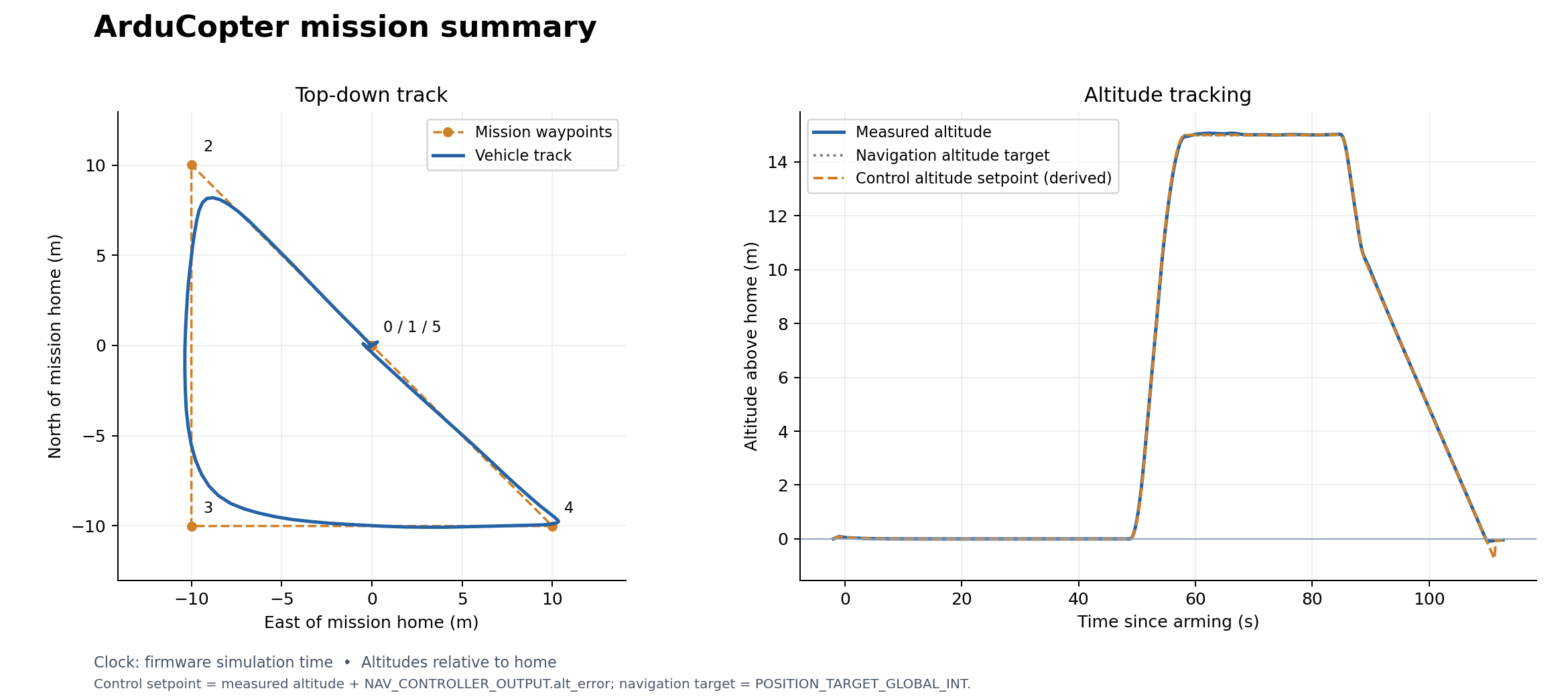
The recorded run completed its waypoints and landed with the same selected controller as the unloaded QAV-R. Explore its measured trajectory and altitude:

Loading constant-load mission…

Static constant-load trajectory and altitude plot

Constant-load mission: trajectory and altitude tracking

Telemetry · Console log · CSV · Run provenance

5. Change an equation, rebuild, and fly

Now model a smoothly varying downward tension, instead of constant weight. This changes the force law while retaining the same motor geometry, firmware, controller, and sensor interface. Create your own source file:

cp modelica/FastDyn/QavrSidePayload.mo modelica/FastDyn/MyLoad.mo

Open modelica/FastDyn/MyLoad.mo in your editor. Rename the opening model QavrSidePayload and closing end QavrSidePayload; to MyLoad. Before the equation section, add:

parameter Real modulation = 0.5 "Fractional change about mean tension";
parameter Real period = 5.0 "Tension period [s]";

Replace the constant force_world equation with:

force_world = {0, 0, -payload_mass * plant.gravity *
  (1 + modulation * sin(2 * pi * time / period))};

Keep period > 0 and 0 <= modulation <= 1. At the defaults, the downward force varies from 0.245 N to 0.735 N, with a mean of 0.49 N. It should be largest at 1.25 s and smallest at 3.75 s. time is simulation time, not wall time; the applied tension also varies before takeoff.

Save this complete overlay as out/my-load.toml:

[FMU]
active = "my_load"

[FMU.models.my_load]
model = "FastDyn.MyLoad"
model_file = "modelica/FastDyn/MyLoad.mo"
source_roots = ["modelica", "third_party/common/modelica_models"]
output = "out/fmi3/MyLoad"
build = true

[FMU.models.my_load.parameters]
payload_mass = 0.05
modulation = 0.5
period = 5.0

Build and check the actual force before flying:

fastdyn-config --base configs/copter462.toml --overlay out/my-load.toml \
  --overlay configs/models/qavr-controller.toml --output out/my-load-run.toml
python utils/build_fmi3_fmu.py --config out/my-load-run.toml --skip-submodules
python tests/integration/payload_model_test.py out/fmi3/MyLoad/FastDyn_MyLoad.fmu
fastdyn run -c out/my-load-run.toml -o out/my-load-run/work

Expect an FMU named FastDyn_MyLoad.fmu, force checks of 0.735, 0.490, 0.245, and 0.490 N at 1.25, 2.5, 3.75, and 5 s, and a mission ending with final landing confirmed near ground. The native check also verifies that the vehicle’s inertial mass remains 0.5 kg and the moment is r × F.

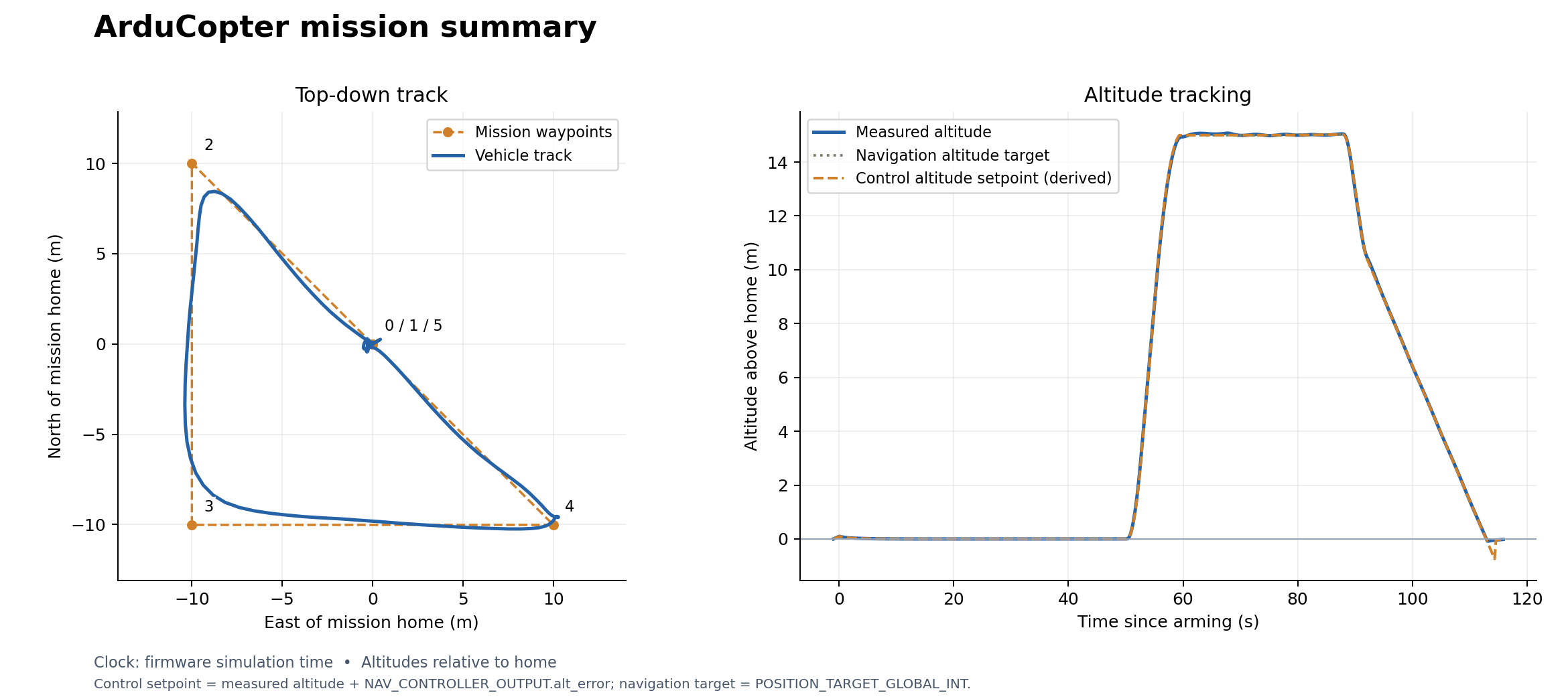
The complete reference implementation is FastDyn.QavrVaryingLoad below. Its recorded mission uses the same new equation and selected gains:

Complete varying-tension model

within FastDyn;

model QavrVaryingLoad "QAV-R with a smoothly varying tension at the front-right motor"
  import Vehicles;
  import Geodesy;
  parameter Real payload_mass = 0.05 "Reference mass for the mean applied weight [kg]";
  parameter Real modulation = 0.5 "Fractional variation about the mean, between 0 and 1";
  parameter Real period = 5.0 "Load period [s], greater than zero";
  // Independent coordinates, matching 0.11 / sqrt(2) at the QAV-R motor.
  parameter Real attachment_b[3] = {0.07778174593052023, -0.07778174593052023, 0}
    "Front-right motor, from CG in body FLU [m]";

  extends Qavr(plant(external_force_b = force_b, external_moment_b = moment_b));

  Real force_world[3] "Prescribed tension in world NWU [N]";
  Real force_b[3] "Applied force in body FLU [N]";
  Real moment_b[3] "Moment about the vehicle CG in body FLU [N*m]";
equation
  assert(period > 0 and modulation >= 0 and modulation <= 1,
    "Use a positive period and modulation between zero and one");
  // Compared with QavrSidePayload, the force law now varies continuously in time.
  force_world = {0, 0, -payload_mass * plant.gravity *
    (1 + modulation * sin(2 * pi * time / period))};
  force_b = transpose(plant.R) * force_world;
  moment_b = cross(attachment_b, force_b);
end QavrVaryingLoad;

Loading varying-load mission…

Static varying-load trajectory and altitude plot

Varying-load mission: trajectory and altitude tracking

Telemetry · Console log · CSV · Run provenance

Compare the two altitude traces and waypoint paths, then change the modulation or period in your overlay and repeat. The native force check verifies the compiled equation at its default parameters, even when the controller rejects much of the disturbance in flight. Keep both run logs; a similar-looking trajectory does not mean the plant stayed the same. This is the edit → compile → check → run → compare workflow to reuse for your own physics.

What this approximation represents

This model exactly describes a prescribed external force at a body attachment point, such as an idealized tension load. Its 0.49 N downward force also equals the weight of 50 g under the model’s 9.8 m/s² gravity, so it approximates that payload’s static hover load.

A real attached payload also resists linear and angular acceleration. A freely hanging payload can swing and change the applied tension. Those effects require additional payload dynamics or changes to the combined mass properties. Keep this exercise focused on an external disturbance; do not use it to claim accurate payload motion during aggressive maneuvers. Next, the payload Monte Carlo study varies this same payload mass while holding the attachment point, vehicle properties, and controller fixed.

Keyboard shortcuts

FastDyn